If you are a Computer Science student or graduate, it is 100% safe to assume this is a subject you absolutely know about.
But if you are currently self-learning programming or a self-taught programmer already in the field like me, there is a chance you may not even heard of this term. But I assure you at one point or another you will face this. When you do, it can be intimidating at first time. To be honest, it was intimidating for me as well - until I decided to go deeper to understand this.
Excerpt from Wikipedia page: https://en.wikipedia.org/wiki/Big_O_notation
Big O notation is a mathematical notation that describes the limiting behavior of a function when the argument tends towards a particular value or infinity. Big O is a member of a family of notations invented by Paul Bachmann,[1] Edmund Landau,[2] and others, collectively called Bachmann–Landau notation or asymptotic notation.
In computer science, big O notation is used to classify algorithms according to how their run time or space requirements grow as the input size grows.[3] In analytic number theory, big O notation is often used to express a bound on the difference between an arithmetical function and a better understood approximation; a famous example of such a difference is the remainder term in the prime number theorem. Big O notation is also used in many other fields to provide similar estimates.
Was this description easy to understand and remember for you? While it is correct, this wasn’t easy for me to make sense of it at first place. Let me share with you the way it made sense to me - I hope it makes sense to you too.
So, What is Big O Notation and why do we need it?
In simple terms, Big O Notation is used to measure performance and scalability of the functions or algorithms we write. In essence it is a mathematical notation as mentioned in Wikipedia article - but you don’t need to be an absolute math wizard to be able to use it.
You may ask, why should I use Big O when there are tools showing how many milliseconds it takes to run a code piece? While it is something handy, it is still not consistent enough for a solid analyze. Because if you have a stronger computer than mine, our times for code execution will not be the same. Even in the same computer times can vary based on how your CPU and RAM performs at that point of time. With Big O, we don’t have to worry about all these details.
When we talk about scalability, we are talking about how much does the function or algorithm slows down as the amount of input grows larger. Let’s say you have an application having 100 users. You use a function to loop through a list of 100 users to get their names. That function will get the job done in a matter of milliseconds.
But what happens when your application grows and you have to go through 10.000, 100.000 or even millions of users? How are we going to figure out what type of data structure and algorithm can efficiently solve this issue? That’s exactly when Big O Notation comes to rescue.
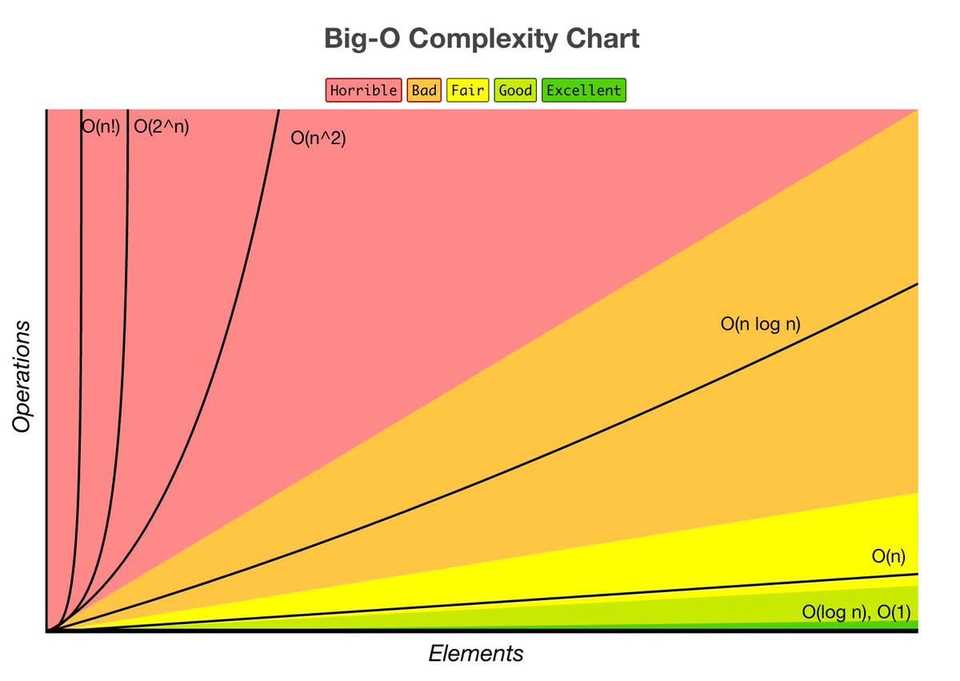
Understanding the Big O complexity graph
- Graph by https://www.bigocheatsheet.com/ -
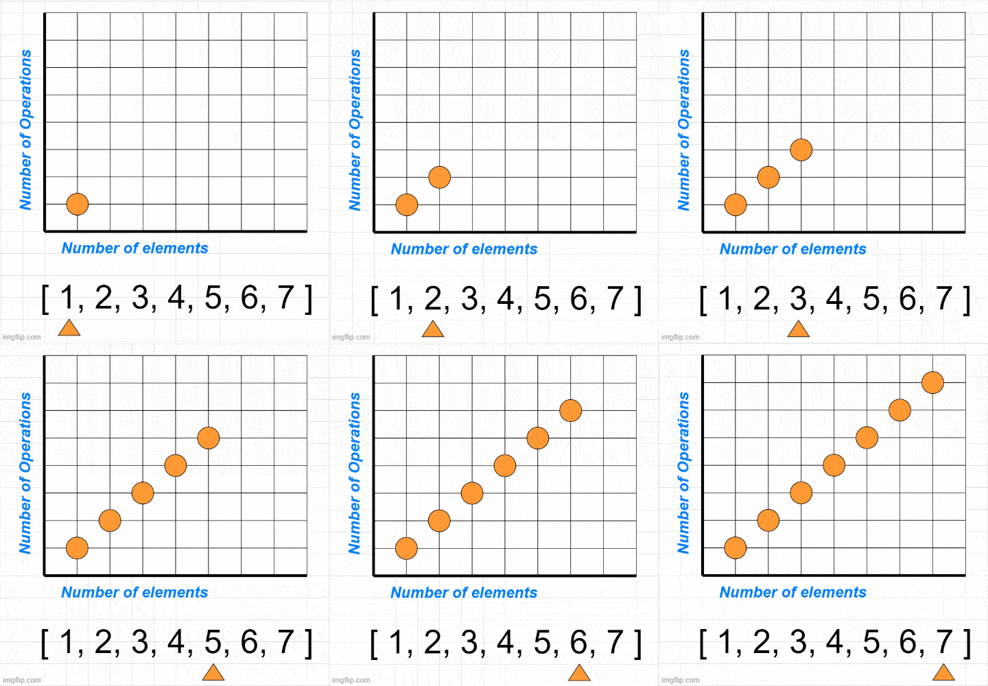
This graph is quite straight-forward about showing what is good or bad with scaling using area colors. But to give you more imagination for the graph, I can share a little interactive gif for you representing this code:
const example = [1, 2, 3, 4, 5, 6, 7]

function printArray (arr) {
  for (let i = 0; i < arr.length; i++) {
    console.log('element:', arr[i])
  }
}

printArray(example)
In the code we simply loop through an array of numbers and printing the each value on console. As you can see in the gif below, number of operations grow respectively with the size of array - because in this code we do one operation per element:

Time and Space complexity
We use Big O to analyze Time and Space complexity of our algorithms. Time and Space are 2 essential metrics to measure for writing efficient code.
Time Complexity: It is related to speed - how long does it take to run the algorithm. Speed is dictated by the CPU (Central Processing Unit) the computer has.
Space Complexity: It is related to memory - how much memory is needed to run the algorithm. This memory here refers to the temporary memory space required by an algorithm to be used, which is called Auxiliary space. Memory is dictated by the RAM (Random Access Memory) the computer has.
Nowadays we have strong computers, but still - our resources are not infinite.
So when you hear about Time and Space complexity next time, remember this: it is about using the resources wisely.
If you are solving a programming problem, there will be a tradeoff between Time and Space.
When you want something to run faster, you may have to tradeoff more memory for it.
When you want something to be cheap in memory, you may have to settle down with lesser speed.
It is an act of balance - different devices, software or platforms will need different type of balance between Time and Space. Having this knowledge as a programmer will help you to be more effective when approaching to problems.
I believe up to this point we have a good ground on definition of Big O, Time & Space complexity and why we need them. Let’s proceed to getting familiar with the most common Big O Notations.
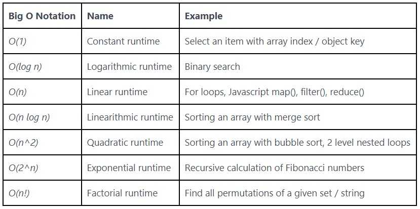
These are the list of complexities we will be covering:
Before I start explaining, I am guessing you must be wondering what does O and numbers or symbols inside paranthesis like (n) stands for.
O refers to the order of the function
(n) represents the number of inputs
O(1) - Constant time
Complexity Rank: Excellent
Constant time is the most optimal complexity when it comes to scaling. Why? Because as the name mentions, it is constant: no matter how many items you need to operate with, amount of time needed to run the algorithm will be exactly the same.
const tenItems = new Array(10).fill('foo')
const millionItems = new Array(1000000).fill('bar')

function returnFirstElement (arr) {
  return arr[0]
}

returnFirstElement(tenItems)
// this will take same amount of time as tenItems array:
returnFirstElement(millionItems)
See? In this case it doesn’t matter how many elements we have. We take the first element and getting done. But keep in mind, constant time is not only about picking only one element. Think it like this: no matter how many inputs we have, amount of operations we do does not change - because it is not dependent on the size of inputs. Check this example:
const tenItems = new Array(10).fill('foo')
const millionItems = new Array(1000000).fill('bar')

function printOnlyFirstFive (array) {
 for (i = 0; i < 5; i++) {
   console.log('element:', array[i])
 }
}

printOnlyFirstFive(tenItems)
// this will take same amount of time as tenItems array:
printOnlyFirstFive(millionItems)
Now you maybe thinking, at first example we did operation with one element so it is O(1). Can we call this O(5) then? Yes, you can count the amount of constants as O(5) - but at the end it is still constant. As a naming convention we will be calling this as O(1) or constant time.
Picking a value from an object via it’s key is also an example of constant runtime. No matter how many elements an object have, amount of time to pick the value is constant:
const todaysMenu = {
  breakfast: 'Smoothie',
  lunch: 'Sallad',
  dinner: 'Sushi',
};

function whatIsInTheMenu(menu, type) {
  return menu[type]
}

whatIsInTheMenu(todaysMenu, 'breakfast') // => Smoothie
Functions like below are also an example for constant runtime algorithms. No matter how big the numbers are, they follow a constant pattern:
function addTen(n) {
  return n + 10
}

console.log(addTen(10)); // => 20
console.log(addTen(1000000)); // => 1000010


function isEvenOrOdd(n) {
  return n % 2 ? 'Odd' : 'Even';
}


console.log(isEvenOrOdd(10)); // => Even
console.log(isEvenOrOdd(10001)); // => Odd
Some examples of constant runtime algorithms:
- Select an element from an array with index number.
- Select an element from an object with key value.
- Check if an item on an array is null.
Some built-in Javascript methods with constant time complexity:
Arrays: push(), pop()
Keep in mind: primitive math operations like sum, multiplication, subtraction, division, modulo, bit shift, etc.. also have a constant runtime.
O(log n) - Logarithmic time
Complexity Rank: Good
Logarithmic runtime algorithms are the next fastest ones after Constant runtime algorithms on scale. Shortest possible explanation would be this: Logarithmic runtime usually applies to algorithms that divides problems in half every step.
A good analogy for this is to think about how you search a word in a dictionary. For example you want to find the word “tree”. You won’t search the word from start by opening every page one by one. Instead you would wide open the pages and go directly to a random page as close as it gets to “T” section. If you go too far, let’s say “U” section - from there you would only try to go back to section “T” only, but not before it.
Typical example for Logarithmic runtime is Binary search. Binary search is an algorithm that finds the location of an argument in a sorted array by dividing the input in half with each iteration. I have specifically highlighted sorted because array should be sorted to get accurate results with this algorithm. Just remember this when you need to use Binary search.
Let’s say we have an array with 10 items and we want to find the item with value 5. What do you do first? Using a for loop, right. Which can be also called a Brute force solution in this situation: we just iterate the array using for loop (linear search):
const tenArray = Array.from(Array(10).keys())

const linearSearch = (arr, target) => {
   for (let i = 0; i < arr.length; i++) {
       if (arr[i] === target) {
           return `Found the target: ${target} at index ${i}`;
       }
   }
}

linearSearch(tenArray, 5)
This will take O(n) - Linear runtime to find the element. You will get more details about this runtime on next chapter - but for the sake of example I will show you below, just know Linear runtime is directly dependent on the length of inputs. Think like this: searching 100 inputs will take 10 times longer than searching 10 items.
Now, let me demonstrate you the scaling difference between Linear Search and Binary Search. I will use Javascript’s performance API to show an approximate comparison. I also encourage you to copy paste this code pieces and try in your favorite code editor.
Again, as I have mentioned before - those numbers can vary based on how strong is your computer. Even on the same computer numbers will be different based on how computer performs at that point of time. Don’t worry if you don’t get the exact same numbers as I have here, what we focus is only how scaling differs between runtimes.
const tenArray = Array.from(Array(10).keys())

// O(n) - LINEAR RUNTIME
const linearSearch = (arr, target) => {
   for (let i = 0; i < arr.length; i++) {
       if (arr[i] === target) {
           return `Found the target: ${target} at index ${i}`;
       }
   }
}

// O(log n) - LOGARITHMIC RUNTIME
const binarySearch = (arr, target) => {
   let startIndex = 0;
   let endIndex = (arr.length)-1;

   while (startIndex <= endIndex){

       let pivot = Math.floor((startIndex + endIndex)/2);

       if (arr[pivot] === target) {
            return `Found the target: ${target} at index ${pivot}`;
       } else if (arr[pivot] < target) {
           startIndex = pivot + 1;
       } else {
           endIndex = pivot - 1;
       }
   }
   return false;
}

let beforeLinear = performance.now()
linearSearch(tenArray, 5)
let afterLinear = performance.now()

let beforeBinary = performance.now()
binarySearch(tenArray, 5)
let afterBinary = performance.now()

console.log('Milliseconds linear search:', afterLinear - beforeLinear)
console.log('Milliseconds binary search:', afterBinary - beforeBinary)

// RESULT:
// => 'Milliseconds linear search:' 0.02500019036233425
// => 'Milliseconds binary search:' 0.06500002928078175
As you see in the example, we have iterated through 10 elements. Linear algorithm performed 2.6 times faster than Logarithmic algorithm. But now let’s see how does the algorithms scale when we iterate through 1 million items:
const millionArray = Array.from(Array(1000000).keys())

// O(n) - LINEAR RUNTIME
const linearSearch = (arr, target) => {
   for (let i = 0; i < arr.length; i++) {
       if (arr[i] === target) {
           return `Found the target: ${target} at index ${i}`;
       }
   }
}

// O(log n) - LOGARITHMIC RUNTIME
const binarySearch = (arr, target) => {
   let startIndex = 0;
   let endIndex = (arr.length)-1;

   while (startIndex <= endIndex){

       let pivot = Math.floor((startIndex + endIndex)/2);

       if (arr[pivot] === target) {
            return `Found the target: ${target} at index ${pivot}`;
       } else if (arr[pivot] < target) {
           startIndex = pivot + 1;
       } else {
           endIndex = pivot - 1;
       }
   }
   return false;
}

let beforeLinear = performance.now()
linearSearch(millionArray, 567841)
let afterLinear = performance.now()

let beforeBinary = performance.now()
binarySearch(millionArray, 567841)
let afterBinary = performance.now()

console.log('Milliseconds linear search:', afterLinear - beforeLinear)
console.log('Milliseconds binary search:', afterBinary - beforeBinary)

// RESULT:
// => 'Milliseconds linear search:' 2.185000106692314
// => 'Milliseconds binary search:' 0.054999953135848045
Now the difference is remarkable. Binary search performed 40 times faster than Linear search when we iterated through 1 million items! But when we used exactly the same functions with 10 items, Linear search was 2.6 times faster than Binary search. I believe this is a great example showing how much difference you can make in the performance by choosing the right algorithm for the problem you want to solve.
O(n) - Linear time
Complexity Rank: Fair
What do we mean when we say linear time? If I tell you all loops we know are an example of linear time complexity / growth, it may start to make more sense.
Because time to finalize going through a loop is directly linked to the length of array. Iterating 100 items will take 10 times longer than iterating 10 items.
const tenItems = new Array(10).fill('foo')
const hundredItems = new Array(100).fill('bar')

function printArray (arr) {
  for (let i = 0; i < arr.length; i++) {
    console.log('element:', arr[i])
  }
}

printArray(tenItems)
// this will take 10 times longer than iterating tenItems array:
printArray(hundredItems)
Some examples to linear runtime algorithms:
- Print all the values in a list.
- Find a given element in a collection.
- Get the maximum or minimum value in an array.
Some built-in Javascript methods with linear time complexity:
Arrays: shift(), unshift(), splice(), concat(), slice(), indexOf(), forEach(), map(), filter(), reduce()
O(n log n) - Linearithmic time
Complexity Rank: Close to fair
Linearithmic time complexity it’s slightly slower than a Linear algorithm - but it is still better than a Quadratic algorithm (which you will see on the next section). O(n log n) is often confused with O(log n). It is a combination of Linear O(n) and Logarithmic O (log n) runtime complexity.
How do they combine? First n is the linear time complexity, which gets multiplied by log n
O(n * log n) -> O (n log n)
Sorting algorithms that utilize a divide and conquer strategy are Linearithmic, such as the following:
Merge sort, Quick sort, Heapsort, Timsort
Let’s take a look at an example, Merge sort:
const someArray = [ 3, 14, 7, 11, 6, 1, 21, 9, 14, 15 ]

// sorting helper:
const merge = (left, right) => {
    let result = [];

    while(left.length || right.length) {

        if(left.length && right.length) {
            if(left[0] < right[0]) {
                result.push(left.shift())
            } else {
                result.push(right.shift())
            }
        } else if(left.length) {
            result.push(left.shift())
        } else {
            result.push(right.shift())
        }
    }
    return result
}

// main function
const mergeSort = (arr) =>{
    if(arr.length <= 1) {
        return arr
    }

    const pivot = arr.length / 2
    const left = arr.slice(0, pivot)
    const right = arr.slice(pivot, arr.length)

  return merge(mergeSort(left), mergeSort(right))
};

mergeSort(someArray)
I won’t be going into detailed analysis of Merge Sort here, but let me give you a simple overview in plain english - so we can look at it’s Big O aspect.
Here is how Merge Sort works:
- It accepts an unsorted array.
- Divides the array smaller pieces one step at a time.
- Sorts them.
- Then merges them back to build a completely sorted array.
- To do this, it recursively uses merge() method we see in the code block. What does recursive mean? In short terms, it is a function calling itself until a condition is met. It is often called as exit condition. As you see above, exit condition is based on the array length.
From the Big O aspect, what do we see:
merge() -> This methods time complexity is based on array length, so it is linear runtime O(n)
mergeSort() -> It divides the array into 2 pieces on each iteration. Remember the Binary Search we discussed about? Merge Sort acts in a similar way here, left and right arrays are cut by half on each iteration. Therefore Logarithmic runtime O(log n) also exists.
At the end, when we merge those 2 functions, we get -> O(n log n)
O(n^2) - Quadratic time
Complexity Rank: Bad
Quadratic is a name to describe squaring - or raising to power of 2. It is literally the good old square of a number in math.
Quick refreshment: What is square of a number? A square of a number is the result of the number multiplied by itself.
Two to the power of two, or 2^2, is the same as 2 * 2, or 4.
5 to the power of 2, or 5^2, is the same as 5 * 5, or 25.
Most classic example for Quadratic runtime is nested loops using the same array. Because you are running a Linear runtime operation within another Linear runtime operation -> O(n * n) = O(n ^ 2)
Let’s see an example:
const fruits = ["apple", "strawberry", "watermelon"]

function logAllPairs(arr) {
  for (i = 0; i < arr.length; i++) {
    for (j = 0; j < arr.length; j++) {
      console.log(`${arr[i]} - ${arr[j]}`)
    }
  }
}

logAllPairs(fruits)

/* Output =>
'apple - apple'
'apple - strawberry'
'apple - watermelon'
'strawberry - apple'
'strawberry - strawberry'
'strawberry - watermelon'
'watermelon - apple'
'watermelon - strawberry'
'watermelon - watermelon'
*/
Here, we use the same array to print out the all pairs. As you see, to get the results from 3 item length array we needed to run 9 times:
3 * 3 or 3 to the power of 2.
What happens if we use 3 nested loops? Can it be still called Quadratic runtime? No. It will be called Cubic runtime, because we will be having O (n ^ 3) or O (n * n * n)
To give you a better picture, functions having Quadratic, Cubic or similar runtimes are also called Polynomial time complexity. Which can be also shown as: O(n ^ k)
n - input
k - power of (2, 3, … any)
Keep in mind: bigger k value will make the algorithm slower. Cubic runtime algorithm will be a lot slower than Quadratic runtime.
O(2^n) - Exponential time
Complexity Rank: Horrible
Exponential or Base 2 means calculations performed by an algorithm doubles everytime as the input grows. We can also say this is the opposite of Logarithmic runtime O(log n) - because on each step calculations are cut by half, while on Exponential it doubles. Typical example for Exponential runtime is calculating Fibonacci numbers recursively. Let me give you a quick overview:
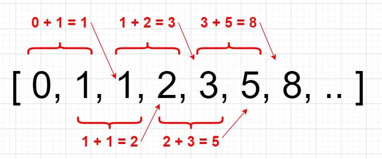
- Fibonacci number is the sum of it’s previous 2 neighbors, starting at 0.
- Just keep in mind - actual calculation starts at third index (or we can say index [2] if we calculate the array starting from index[0]). Because it’s the first index that has 2 previous neighbors:
- With the following function, we will give an index number to return the nth Fibonacci number in the sequence using recursion. This solution is also called “naive” solution for this problem, I suggest you to check and study optimized solutions for finding Fibonacci number. For now, we only want to focus on the Big O aspect here:
function fibonacciRecursive(num) {
  // exit conditions, return if it is 0 or 1
  if (num === 0) return 0
  else if (num === 1) return 1
  // else, call the function recursively
  else return fibonacciRecursive(num - 1) + fibonacciRecursive(num - 2)
}

fibonacciRecursive(4)
// OUTPUT => 3
What happens here? When we run the function, we get multiple returned recursive results. At each step amount of calculation doubles!
fibonacciRecursive(4) = fibonacciRecursive(3) + fibonacciRecursive(2)
fibonacciRecursive(3) = fibonacciRecursive(2) + fibonacciRecursive(1)
fibonacciRecursive(2) = fibonacciRecursive(1) + fibonacciRecursive(0)
// fib(1) and fib(0) are 0 and 1 respectively
Pop out from the stack:
fibonacciRecursive(2) = 1 + 0 = 1
fibonacciRecursive(3) = 1 + 1 = 2
fibonacciRecursive(4) = 1 + 2 = 3
Time complexity scales very quickly. See, we are calling the fibonacci(2) and fibonacci(1) twice.
You should avoid functions with Exponential runtimes if it is possible, since their scaling is awful. But this is not the worst one yet. There is one time complexity left we need to take a look on the next section.
O(n!) - Factorial time
Complexity Rank: Worst
Factorial is a number, which is result of multiplication of all positive integer numbers up to that number.
6! = 6 x 5 x 4 x 3 x 2 x 1 = 720
See? It grows extremely fast.
Classical example for usage of Factorial runtime is the Travelling Salesman problem. Let’s say you are a sales person and you have to visit n number of cities. What would be the shortest route that visits each city, then returns you to the place where you started? To solve this problem, we need to calculate every possible route. That’s when permutations comes into the picture.
You need to visit 3 cities this week. How many permutations do we have?
function getPermutations (arr) {
  if (arr.length <= 2) {
    if (arr.length === 2) return [arr, [arr[1], arr[0]]]
    return arr
  }
  return arr.reduce(
    (acc, item, i) =>
      acc.concat(
        getPermutations([...arr.slice(0, i), ...arr.slice(i + 1)]).map(val => [
          item,
          ...val,
        ])
      ),
    []
  );
}

const cities = ['Copenhagen','Stockholm', 'Oslo']
getPermutations(cities)
This is factorial 3, or 3!, returns 6 different routes:
[
  [ 'Copenhagen', 'Stockholm', 'Oslo' ],
  [ 'Copenhagen', 'Oslo', 'Stockholm' ],
  [ 'Stockholm', 'Copenhagen', 'Oslo' ],
  [ 'Stockholm', 'Oslo', 'Copenhagen' ],
  [ 'Oslo', 'Copenhagen', 'Stockholm' ],
  [ 'Oslo', 'Stockholm', 'Copenhagen' ]
]
What happens if you need to calculate permutations for 18 cities? It would be 18! Factorial.
Which will be 6,402,373,705,728,000 different routes!
You want to stay away from algorithms having this runtime if possible. To optimize this type of problems, I suggest you to research about Heuristic algorithms.
I hope this article helped you to understand Big O Notation concept and made you familiar with the common Big O runtime complexities. Thanks for reading!


